This is the capstone project required to get the IBM Data Science Professional Certificate. Yan Luo, a data scientist and developer, and Joseph Santarcangelo, both data scientists at IBM, directed the project. The project will be presented in seven sections, and the lecture Jupyter notebooks and tutorials were used to compile the contents.

As a data scientist, I was tasked with forecasting if the first stage of the SpaceX Falcon 9 rocket will land successfully, so that a rival firm might submit better informed bids for a rocket launch against SpaceX. On its website, SpaceX promotes Falcon 9 rocket launches for 62 million dollars, whereas other companies charge upwards of 165 million dollars. A significant portion of the savings is attributable to SpaceX's ability to reuse the first stage. If we can determine whether the first stage will land, we can calculate the launch cost. This information might be useful if an alternative company want to compete with SpaceX for a rocket launch. In this project, I will conduct data science methodology including business understanding, data collection, data wrangling, exploratory data analysis, data visualization, model development, model evaluation, and stakeholder reporting.

In the final section, we will apply machine learning models to the dataframes on which we have already conducted feature engineering (in the fifth section). Initially, we will standardize the data and split it into training data and test data; next, using four different machine learning techniques (logistic regression, support vector machine (SVM), decision tree classifier, and k-nearest neighbors classifier (KNN)), we will generate predictions to determine whether the first stage SpaceX Falcon 9 will land successfully or not. During the training of the ML algorithms, we will use GridSearchCV to identify the hyperparameters that provide our machine learning models the highest level of accuracy while preventing overfitting.

We will utilize scikit-learn (sklearn), the most popular and powerful Python library for machine learning. It offers a variety of effective methods for machine learning and statistical modeling, such as classification, regression, clustering, and dimensionality reduction, through a Python interface that is consistent. The NumPy, SciPy, and Matplotlib packages form the foundation of this Python-based library.

We start by importing the necessary Python package for this section.

import pandas as pd
import numpy as np
import matplotlib.pyplot as plt
import seaborn as sns

from sklearn import preprocessing
from sklearn.model_selection import train_test_split
from sklearn.model_selection import GridSearchCV

from sklearn.linear_model import LogisticRegression
from sklearn.svm import SVC
from sklearn.tree import DecisionTreeClassifier
from sklearn.neighbors import KNeighborsClassifier

Next, we define a function employing the seaborn library to plot the confusion matrices in order to evaluate the classification results of model predictions for rocket landings.

def plot_confusion_matrix(y,y_predict):
    "this function plots the confusion matrix"
    from sklearn.metrics import confusion_matrix

    cm = confusion_matrix(y, y_predict)
    ax= plt.subplot()
    sns.heatmap(cm, annot=True, ax = ax); #annot=True to annotate cells
    ax.set_xlabel('Predicted labels')
    ax.set_ylabel('True labels')
    ax.set_title('Confusion Matrix'); 
    ax.xaxis.set_ticklabels(['did not land', 'land']); ax.yaxis.set_ticklabels(['did not land', 'landed']) 
    plt.show() 

Two dataframes from the fifth section will be employed. Initially, we import the dataframe including the "Class" column prior to one-hot encoding.

URL1 = "https://cf-courses-data.s3.us.cloud-object-storage.appdomain.cloud/IBM-DS0321EN-SkillsNetwork/datasets/dataset_part_2.csv"

data = pd.read_csv(URL1)
data.head()

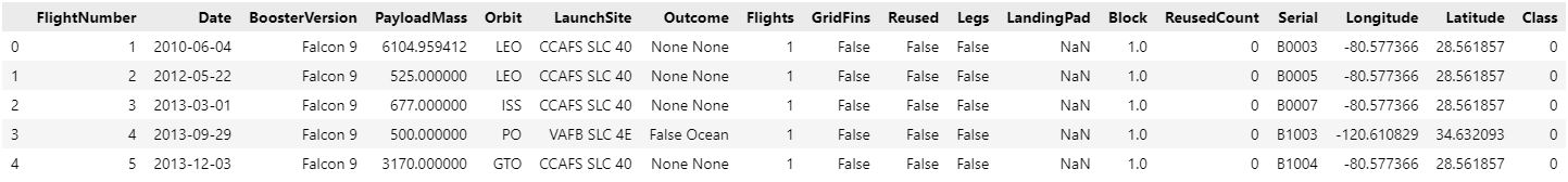
We set the attributes of the "Class" column as target variables Y for machine learning models, and convert it to numpy format.

Y = data['Class'].to_numpy()

Second, we import the one-hot encoded dataframe to use its variables as X values that are correlated with Y values in order to make predictions.

URL2 = 'https://cf-courses-data.s3.us.cloud-object-storage.appdomain.cloud/IBM-DS0321EN-SkillsNetwork/datasets/dataset_part_3.csv'
X = pd.read_csv(URL2)
X.head()

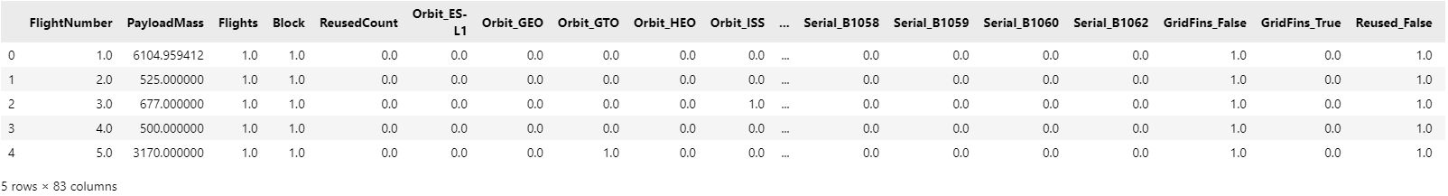
To utilize this dataframe, we need to standardize its features such that they all contribute equally to the predictions.

transform = preprocessing.StandardScaler()
X = transform.fit_transform(X)

Next, we use the function train_test_split to split the data X and Y into training and test data. We set the parameters test_size to 0.2 and random_state to 2 to use 20% of the data as a test dataset and to have the same results when we choose random state 2. We can see the number of samples for each set separately.

transform = X_train, X_test, Y_train, Y_test = train_test_split(X, Y, test_size=0.2, random_state=2)

print(X_train.shape, X_test.shape, Y_train.shape, Y_test.shape) 

In this phase, we will train four different ML models and try to optimize their accuracy. To do that, we will use the GridSearchCV function while training our models so that cross-validation is performed along with GridSearchCV to optimize hyperparameters. Cross-validation is used while training the model, so before training the model with data, we divide the data into two parts: train data and test data. The algorithm trains and validates the model by comparing the accuracy results of each fold defined with the CV parameters of the GridSearchCV function. We can also define values for different parameters of each ML model to automatically select the best value for the corresponding parameter to optimize the accuracy of our models. We will explain different hyperparameters for each corresponding ML model.

To begin with, we create a logistic regression object and a parameter dictionary to define them later as the parameters of GridSearchCV.

Then, we make a GridSearchCV object using the logistic regression algorithm as the estimator and the parameters dictionary to list the hyperparameters. We also set the cv parameter to 10 to have 10 folds to train and validate our model.

Lastly, we use the X_train and Y_train datasets to fit GridSearchCV object for logistic regression. We display the best parameters using the data attribute best_params_ and the accuracy on the validation data using the data attribute best_score_.

lr=LogisticRegression()
parameters ={"C":[0.01,0.1,1],'penalty':['l2'], 'solver':['lbfgs']}

logreg_cv = GridSearchCV(lr, parameters, cv=10)
logreg_cv.fit(X_train, Y_train)

print("tuned hyperparameters :(best parameters) ",logreg_cv.best_params_)
print("accuracy :",logreg_cv.best_score_)

To evaluate the accuracy of the trained model, we can calculate the accuracy on the test data using the GridSearchCV method score.

acc_logreg_test_data = logreg_cv.score(X_test, Y_test)
print("Accuracy on test data :", acc_logreg_test_data)

Another method to evaluate the accuracy of the trained model is examining the confusion matrix. We can plot the confusion matrix on the test data by using the following syntax. We generates predictions for X_test data and use it to compare with actual values on a confusion matrix.

yhat=logreg_cv.predict(X_test)
plot_confusion_matrix(Y_test,yhat)

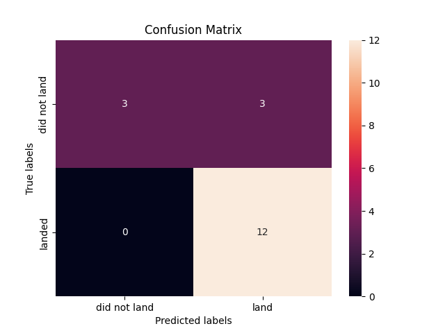
The confusion matrix demonstrates that the logistic regression model can differentiate between classes. The primary issue is false positives. The classifier considers an unsuccessful landing as a successful landing.

Support vector machine (SVM) is the second model that will be trained. We will construct an SVM object and a parameter dictionary to define the GridSearchCV function's SVM hyperparameters.

The SVM algorithm is used as the estimator, and the parameters dictionary is used to store the hyperparameters, before a GridSearchCV object is created. In addition, we trained and tested our model using 10 separate datasets (folds) by setting the CV parameter to 10.

The GridSearchCV object is then fitted for an SVM model using the X_train and Y_train datasets. Using the data attribute best params , we provide the optimal parameters, and using the data attribute best score , we display the accuracy on the validation data.

parameters = {'kernel':('linear', 'rbf','poly','rbf', 'sigmoid'),
	'C': np.logspace(-3, 3, 5),
	'gamma':np.logspace(-3, 3, 5)}

svm = SVC()

svm_cv = GridSearchCV(svm, parameters ,cv=10)
svm_cv.fit(X_train,Y_train)

print("tuned hyperparameters :(best parameters) ",svm_cv.best_params_)
print("accuracy :",svm_cv.best_score_)

The score method of GridSearchCV function allows us to compute the accuracy on the test data, allowing us to assess the trained model's performance.

acc_svm_test_data = svm_cv.score(X_test, Y_test)
print("Accuracy on test data :", acc_svm_test_data)

The confusion matrix can also be used as a measure of the trained model's accuracy. With the following syntax, we can visualize the confusion matrix for the test data. We create predictions for the X test dataset and then use the confusion matrix to compare these predictions to the actual values.

yhat=svm_cv.predict(X_test)
plot_confusion_matrix(Y_test,yhat)

The SVM model's ability to distinguish between classes is illustrated by the confusion matrix. False positive results are the main problem. An unsuccessful landing is treated as a successful one by the classifier.

We start by building a decision tree classifier object and a dictionary of parameters. GridSearchCV's parameters will subsequently be defined using the dictionary.

Next, we generate a GridSearchCV object with the parameters dictionary listing the hyperparameters and the decision tree classifier algorithm as the estimator. We used 10 folds for model training and validation, which was achieved by setting the CV parameter to 10.

After that, we employ the X_train and Y_train datasets to fit the GridSearchCV object to the decision tree classifier model. We provide the best parameters by means of the data attribute best_params_  and the accuracy of the validation data by means of the data attribute best_score_.

parameters = {'criterion': ['gini', 'entropy'],
     'splitter': ['best', 'random'],
     'max_depth': [2*n for n in range(1,10)],
     'max_features': ['auto', 'sqrt', 'log2'],
     'min_samples_leaf': [1, 2, 4],
     'min_samples_split': [2, 5, 10]}

tree = DecisionTreeClassifier()

tree_cv = GridSearchCV(tree, parameters, cv=10)
tree_cv.fit(X_train, Y_train)

print("tuned hpyerparameters :(best parameters) ",tree_cv.best_params_)
print("accuracy :",tree_cv.best_score_)

The GridSearchCV method score can be used to measure the accuracy of the trained model by calculating its accuracy on the test data.

acc_tree_test_data = tree_cv.score(X_test, Y_test)
print("Accuracy on test data :", acc_tree_test_data)

Examining the confusion matrix is another way for assessing the accuracy of the trained model. We can plot the confusion matrix using the below syntax on the test data. We construct predictions for the X_test data and use a confusion matrix to compare them to the actual values.

yhat = tree_cv.predict(X_test)
plot_confusion_matrix(Y_test,yhat)

The confusion matrix shows that the decision tree classifier can distinguish between classes. False-positives are the key issue. A failed landing is considered a successful landing by the classifier.

Initially, we construct a k-nearest neighbors classifier object and a parameter dictionary in order to later describe them as the parameters of GridSearchCV.

The k-nearest neighbors classifier algorithm is next used as the estimator, and the parameters dictionary is used to specify the hyperparameters when we create a GridSearchCV object. We used 10 folds for model training and validation, which was achieved by setting the cv parameter to 10.

We next utilize the X train and Y train datasets to fit the GridSearchCV object to the k-nearest neighbors classifier model. We provide the finest parameters via the data attribute best_params_ and the validation data's accuracy via the data attribute best_score_.

parameters = {'n_neighbors': [1, 2, 3, 4, 5, 6, 7, 8, 9, 10],
	'algorithm': ['auto', 'ball_tree', 'kd_tree', 'brute'],
	'p': [1,2]}

KNN = KNeighborsClassifier()

knn_cv = GridSearchCV(KNN, parameters, scoring='accuracy', cv=10)
knn_cv = knn_cv.fit(X_train, Y_train)

print("tuned hpyerparameters :(best parameters) ",knn_cv.best_params_)
print("accuracy :",knn_cv.best_score_)

The GridSearchCV method score can be used to compute the accuracy of the trained model on test data for evaluation.

acc_knn_test_data = knn_cv.score(X_test, Y_test)
print("Accuracy on test data :", acc_knn_test_data)

Examining the confusion matrix is another way to evaluate the trained model's accuracy. The following syntax allows us to plot a confusion matrix over the test dataset. We then use a confusion matrix to compare our predicted values to the actual values of the X_test data.

yhat = knn_cv.predict(X_test)
plot_confusion_matrix(Y_test,yhat)

The confusion matrix proves that the k-nearest neighbor classifier is effective at making distinctions between classes. False positives are the main problem. A landing that isn't successful is nonetheless counted as a success by the classifier.

For the test dataset, each machine learning model achieved the same accuracy score, and their confusion matrices are also identical. Using the best score attribute of the GridSearchCV function, we will employ a syntax that compares and returns the ML model with the highest accuracy score for predicting the outcome of a rocket landing. Then, we will display the parameters of the selected algorithm using the best params attribute of the GridSearchCV function so that we have the name of the best classification algorithm as well as the hyperparameters to utilize for predicting SpaceX's Falcon 9 First Stage Landing.

algorithms = {'KNN':knn_cv.best_score_,'Tree':tree_cv.best_score_,'LogisticRegression':logreg_cv.best_score_}
best_algorithm = max(algorithms, key=algorithms.get)
print('Best Algorithm is',best_algorithm,'with a score of',algorithms[best_algorithm])
if best_algorithm == 'Tree':
	print('Best Params is :',tree_cv.best_params_)
if best_algorithm == 'KNN':
	print('Best Params is :',knn_cv.best_params_)
if best_algorithm == 'LogisticRegression':
	print('Best Params is :',logreg_cv.best_params_)

According to our results, the Decision Tree Classifier Algorithm is the most effective machine learning technique for our project. The best parameters to use are 'gini' for criterion, 6 for max_depth, 'auto' for max_features, 4 for min_samples_leaf, 5 for min_samples_split and 'best' for splitter.